Examples

\[\]

3D Deconvolution

We consider the C. elegans embryo real dataset (\(672 \times 712 \times 104 \)) that can be downloaded here and that is shown in Figure 1. This sample contains

• nuclei (DAPI channel-blue)

• protein spots (CY3 channel-red)

• microtubules (FITC channel-green).

The PSF for each channel, generated from a theoretical model, is also provided here. In what follows, each channel is deconvolved separately using the same code.

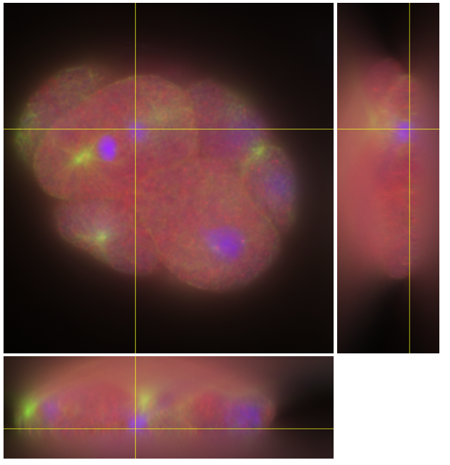
Fig 1. C. Elegans embryo. Blue: chromosomes in the nuclei. Green: microtubules. Red: a protein stained with CY3.

We start by reading the data

%% Reading data
psf=double(loadtiff(psfname));psf=psf/sum(psf(:));
y=double(loadtiff(dataname));maxy=max(y(:));y=y/maxy;
sz=size(y);

We then resize the PSF and enforce compliance with the periodic assumption of the FFT. This is particularly relevant in the axial direction where there is signal at the boundaries of the volume. Note that the function fft_best_dim (Util/ folder) returns sizes that are suited to efficient FFT operations.

padsz=[0,0,52];
sznew=fft_best_dim(sz+2*padsz);
halfPad=(sznew-sz)/2;
psf=padarray(psf,halfPad,0,'both');

We now define our data-fidelity term, TV regularization, and nonnegativity constraint.

%% Least-squares data-fidelity term
H=LinOpConv(fftn(fftshift(psf)));                      % Convolution operator
H.memoizeOpts.apply=true;
S=LinOpSelectorPatch(sznew,halfPad+1,sznew-halfPad);   % Selector operator
L2=CostL2(S.sizeout,y);                                % L2 cost function
LS=L2*S;                                               % Least-squares data term
%% TV regularization
Freg=CostMixNorm21([sznew,3],4);      % TV regularizer: Mixed norm 2-1
Opreg=LinOpGrad(sznew);               % TV regularizer: Operator gradient
Opreg.memoizeOpts.apply=true;
lamb=2e-6;                            % Regularization parameter
%% Nonnegativity constraint
pos=CostNonNeg(sznew);                % Nonnegativity: Indicator function
Id=LinOpIdentity(sznew);              % Identity operator

Here, our cost function is $$ \mathcal{C}(\mathrm{x}) = \frac12 \|\mathrm{SHx - y} \|_2^2 + \lambda \|\nabla \mathrm{x} \|_{2,1} + i_{\geq 0}(\mathrm{x}),$$ where \(\lambda >0\) is the regularization parameter, \(\mathrm{S}\) an operator that selects the “unpadded” (valid) part of the convolution result \(\mathrm{Hx}\), and the two other terms are the TV regularization and the nonnegativity constraint, respectively. We are now ready to instanciate and run our algorithm (here, ADMM) to minimize our functional.

dispIt=30;                     % Verbose every 30 iterations
maxIt=300;                     % Maximal number of iterations
Fn={LS,lamb*Freg,pos};         % Functionals F_n constituting the cost
Hn={H,Opreg,Id};               % Associated operators H_n
rho_n=[1e-3,1e-3,1e-3];        % Multipliers rho_n
ADMM=OptiADMM([],Fn,Hn,rho_n); % Declare optimizer
ADMM.OutOp=OutputOpti(1,[],round(maxIt/10),[1 2]); % build the output object
ADMM.CvOp=TestCvgCombine(TestCvgCostRelative(1e-4), 'StepRelative',1e-4); % Set the convergence tests
ADMM.ItUpOut=dispIt;
ADMM.maxiter=maxIt;
ADMM.run(zeros(sznew));

Here, three splittings have been done: \(\mathrm{u_1=Hx}, \; \mathrm{u_2=\nabla x}\), and \(\mathrm{u_3=x}\). We do not need to provide a solver to the ADMM algorithm (5th argument) since the operator algebra ensures that the operator $$\rho_1 \mathrm{H^*H} + \rho_2 \nabla^* \nabla + \rho_3 \mathrm{I}$$ results in a LinOpConv that is invertible. Hence, ADMM builds this operator automatically and uses its inverse for the linear step of the algorithm (minimization over \(\mathrm{x}\)).

The deconvolved image is shown in Figure 2.

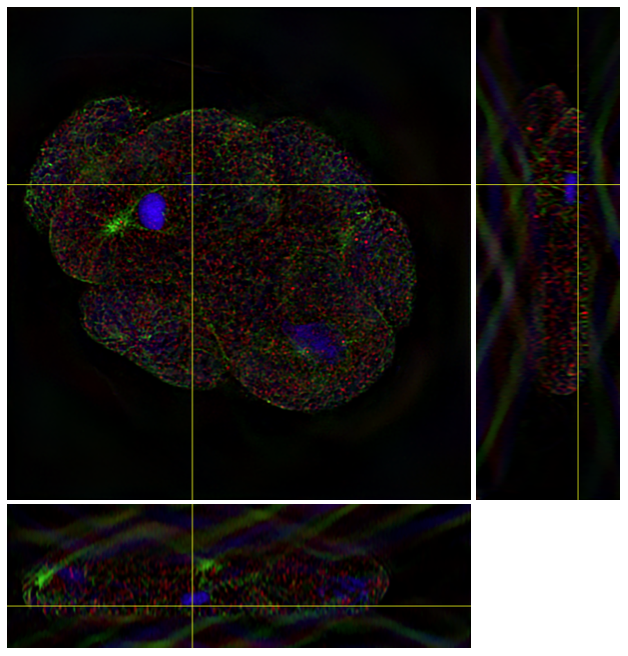
Fig 2. Deconvolved C. Elegans embryo.