Directional analysis of 2D images — ImageJ/Fiji plugins
August 2026

How to use
Open a 2D grayscale image and pick a command under Plugins ▸ OrientationJ. Whatever the command, the computation is the same: a gradient is taken at every pixel, the gradient structure tensor is averaged over a local window, and its eigen-analysis gives the orientation, the coherency and the energy. Two settings govern the measurement itself — the analysis scale σ and the gradient — and both appear in the Structure Tensor block of every dialog; each command then adds its own options, such as the coherency and energy thresholds of Distribution or the grid of Vector Field.
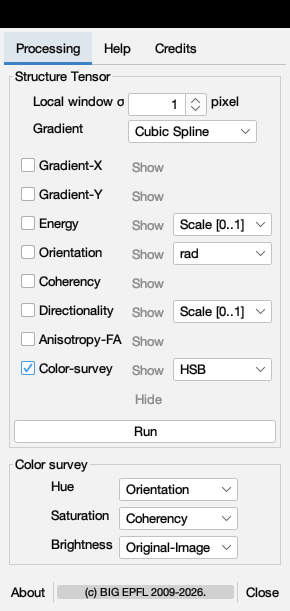
The Analysis dialog, shown here, is representative of all of them. The upper block sets σ ("Local window") and the gradient, then selects which feature maps to produce. Energy and directionality are unbounded, so they carry a display scaling — Scale [0..1] for a normalized view, No scale for the raw values you want to measure; coherency and anisotropy are already in [0, 1] and are shown as computed. The lower block builds the color survey: which feature drives the hue, the saturation and the brightness. Every field has a macro equivalent, so once a setting works it can be recorded and replayed over a whole folder.
Select the scale σ
σ is the standard deviation, in pixels, of the Gaussian window over which the tensor is averaged. It is the most consequential choice: it defines what local means, and therefore which structures the measurement describes.
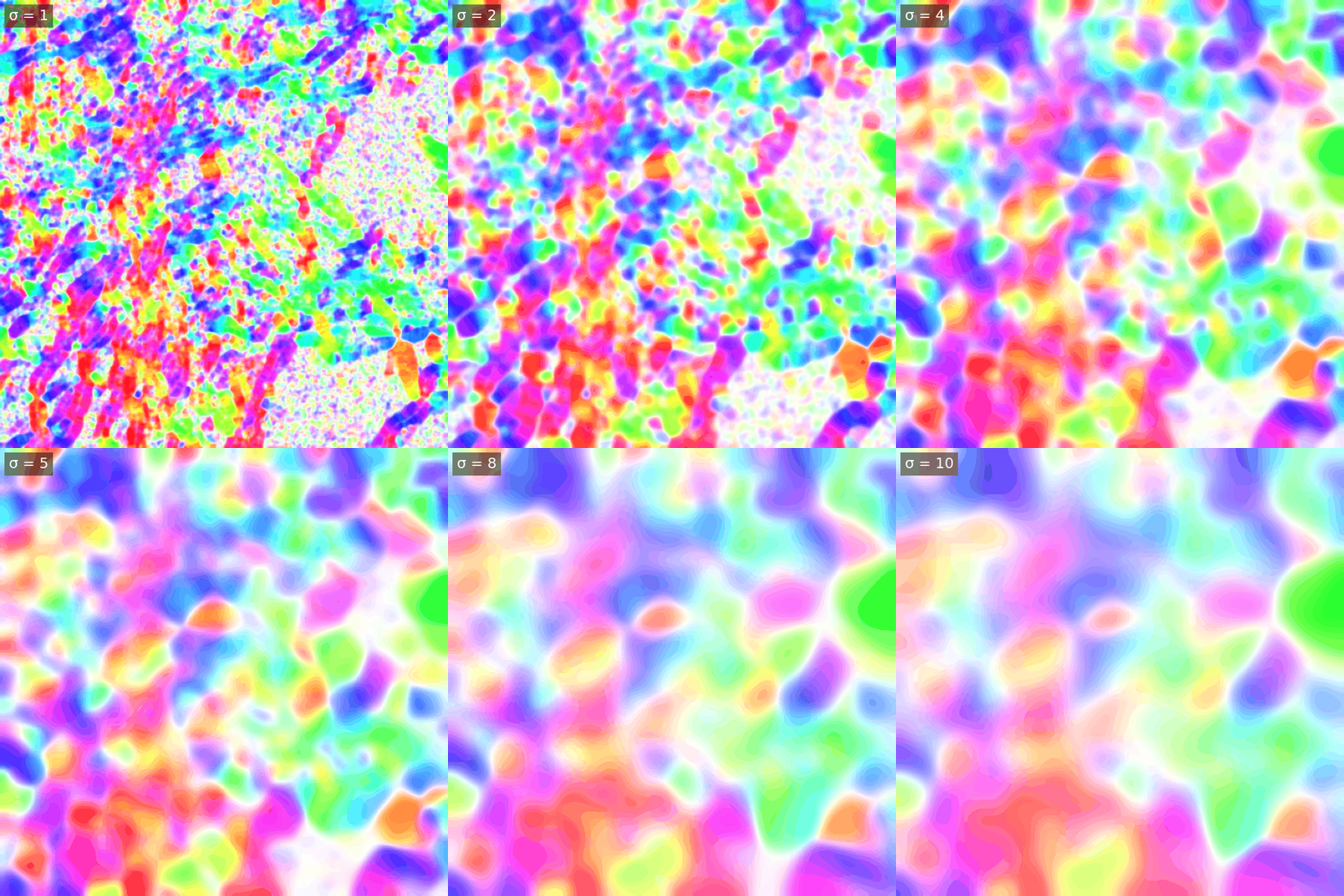
The same collagen field analyzed with a growing window. A small σ resolves individual fibers and reacts to noise; a large σ merges neighbors into a smooth regional trend.
Two rules of thumb:
- Match the structure width. Start with σ of about half the width of the fibers or stripes of interest — σ = 1–2 px for thin fibers, more for coarse bundles.
- Know what you trade. A small σ follows fine detail but yields noisy angles and low coherency everywhere; a large σ gives stable, smooth angles but blends neighboring structures and rounds corners. When structures live at several scales, analyze at several σ and compare: the coherency map tells you at which scale each region is best described.
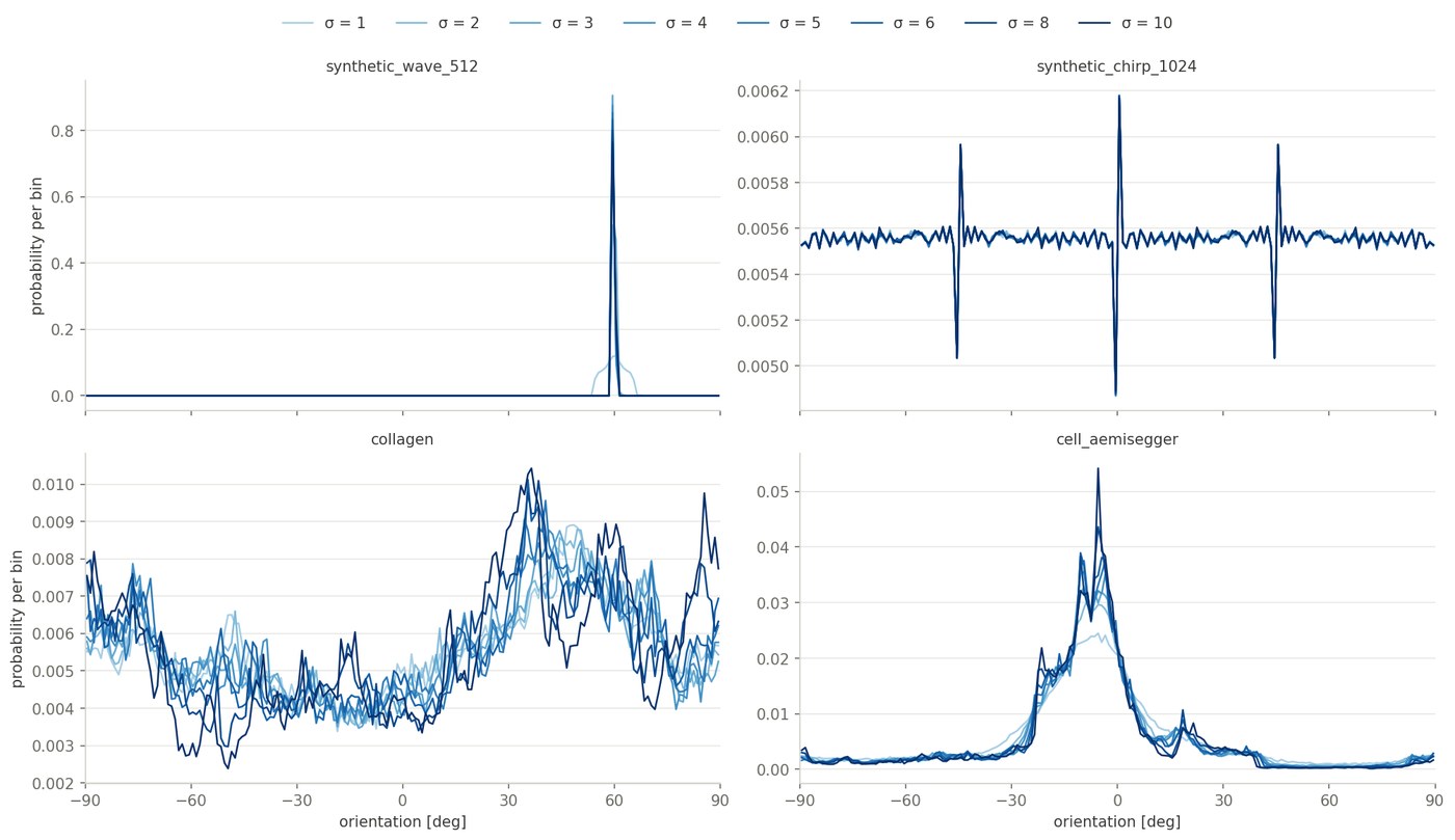
The effect is easiest to read on the angular histogram, where a growing σ sharpens a well-defined peak and suppresses the background spread:
Select the gradient
The gradient decides how the derivatives are estimated before the tensor is assembled. On a chirp, whose local period is known everywhere, the differences are measurable:
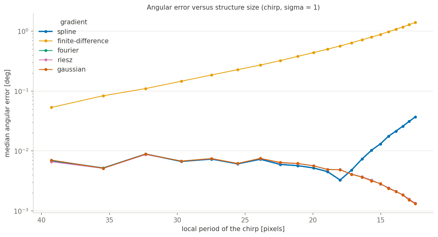
- Cubic Spline (the default) — the exact derivative of the cubic-spline interpolation of the image: accurate down to fine structures, and the setting used throughout this documentation. Keep it unless you have a reason not to.
- Finite Difference — the simplest and fastest, but one to two orders of magnitude more biased, increasingly so as structures get finer.
- Fourier, Riesz and Gaussian — band-limited derivatives that stay accurate at small periods, useful on noisy or oscillating data, at the cost of spatial locality (Fourier can ring near the borders).
Analysis
Produces the feature maps — orientation, coherency, energy, directionality, anisotropy — and the color survey, which paints them over the image: hue for the orientation, saturation for the coherency, brightness for the original intensity. Flat and isotropic regions therefore stay gray, and only genuinely oriented structures take on color.
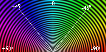
The color coding of the orientation: green at 0°, blue at +45°, orange at −45°, red at ±90°.
Distribution
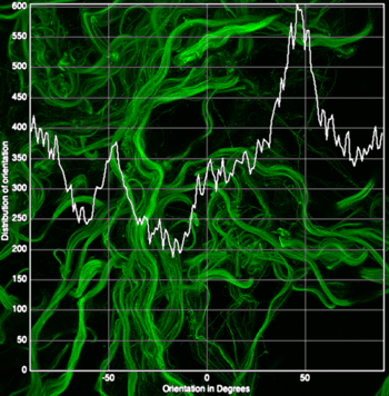
Bins the local orientations into an angular histogram, with minimum-coherency and minimum-energy thresholds so that only meaningful pixels are counted. This is the command most often used to quantify alignment, and its table can be exported for statistics.
Vector Field
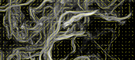
Overlays one vector per grid cell, with a length that is constant or scaled by energy, coherency, or both. The most readable summary for a figure, though the histogram is the better instrument for quantification.
Measure
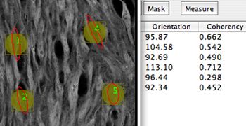
Reports orientation, coherency and energy inside the current selections, as a table — the tool for comparing a few regions rather than mapping the whole field.
Dominant Direction
Collapses the whole image to a single angle with its coherency: a one-number answer, convenient for batch comparisons across a series.
Clustering
Groups locally oriented regions into clusters and reports one representative vector per cluster — position, direction, coherency, energy — a structure-level summary of the vector field.
Horizontal Alignment
Rotates each slice of a stack so that its dominant direction becomes horizontal, which registers fibrous samples acquired at arbitrary angles before further analysis.
Test Image
Generates the calibration patterns the documentation uses: a radial chirp, whose local period sweeps across the field, and a stack of oriented patterns — in small, large and custom sizes. The fastest way to check an installation, and the reference material for choosing σ and the gradient.
MonogenicJ
A companion plugin, on a different footing: instead of one local window it builds a multiresolution monogenic representation of the image with the Riesz–Laplace wavelet transform, and reports orientation, coherency and phase at every scale. Use it when the structures of interest live at several scales at once. Details on the MonogenicJ page.
Corner Harris
Harris keypoint detection, built on the same structure tensor: corners are the places where both eigenvalues are large.