Fiji/ImageJ plugins — Directional Image Analysis (2D)

Daniel Sage · Center for Imaging and Biomedical Imaging Group, Ecole Polytechnique Fédérale de Lausanne (EPFL)

Compare gradients

Before any tensor is assembled, the image has to be differentiated — and the way that derivative is computed is a choice, not a detail. OrientationJ offers five:

gradient	how the derivative is taken
Cubic spline (default)	the exact derivative of the cubic-spline interpolation of the image
Finite difference	the difference of neighboring pixels, the cheapest estimate
Fourier	multiplication by iω in the frequency domain, exact for a band-limited image
Riesz	the Riesz transform, a band-limited derivative with a smoother spectral profile
Gaussian	convolution with the derivative of a Gaussian, which smooths as it differentiates

They differ in how far they reach around a pixel, and therefore in what they can resolve: the wider the support, the better the behavior at fine structures and the worse the locality. This page measures that trade-off, at structure-tensor window σ = 1, on images whose answer is known — analytically, or by construction.

Error against the size of the structures

On the radial chirp, whose period grows from the center outwards, the true orientation is tangential everywhere, so the angular error can be plotted against the local period. This is the measurement that decides the default:

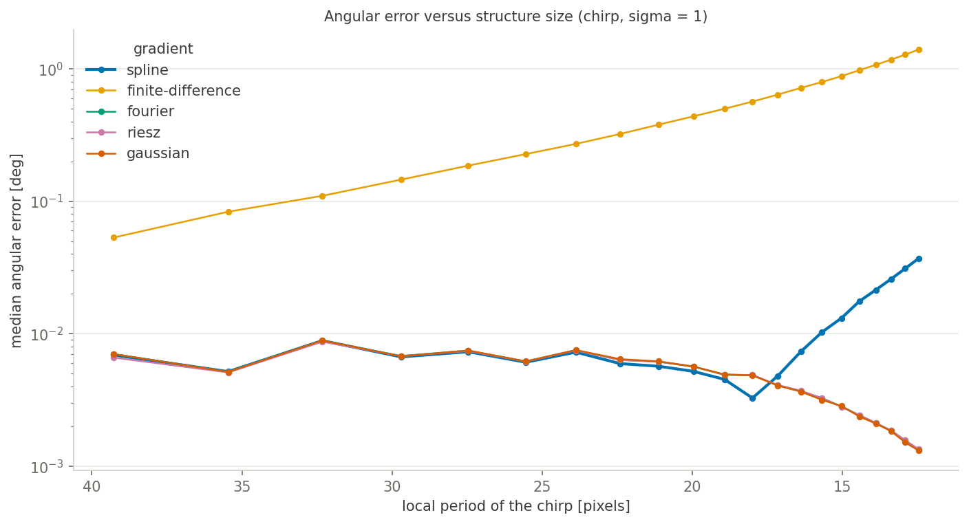
Every gradient converges once the structures are comfortably sampled. They part company below about ten pixels per period: the finite difference degrades first and worst, one to two orders of magnitude above the others, while the band-limited derivatives — Fourier, Riesz, Gaussian — and the cubic spline hold their accuracy down to the sampling limit.

Two orientations at two scales

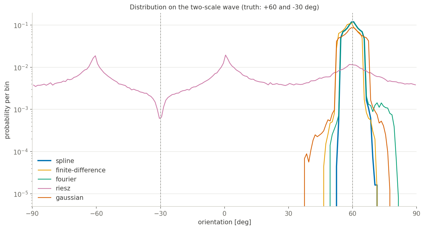
The wave image carries fringes at exactly +60° and −30°, of two different periods, so a gradient can be wrong on one and right on the other. The histograms show which:

Bias where there is no orientation

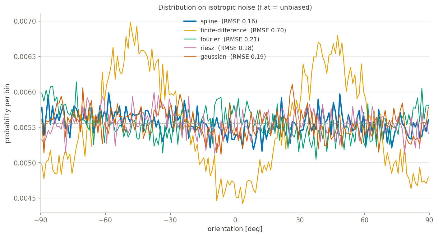
Isotropic noise has no preferred direction, so the distribution of the measured angles must be flat. Any structure in it is bias introduced by the derivative itself, and the separable finite difference is the one that shows it, favoring the axes of the pixel grid:

What to choose

Keep the cubic spline: it is accurate down to fine structures, unbiased on isotropic data, and local. Take Fourier or Riesz when the structures approach the pixel and the image is band-limited and free of border artifacts, and Gaussian when the data is noisy and a little smoothing is welcome — it is also the gradient of the minimal operator. Avoid the finite difference unless speed outweighs everything: it is the only one that is both biased on noise and inaccurate on fine structures.

Files

file	content
gradients.ipynb	angular errors, error versus period, isotropy and wave figures, conclusion
macro-gradients.ijm	Fiji macro — OrientationJ Analysis with each gradient, saves the orientation maps