Structure tensor vs nematic tensor¶

OrientationJ measures the local orientation with the gradient structure tensor. Two other estimators are built from the very same gradient and the very same window, and differ only in the weight they give to each pixel. This assessment measures the three on an image whose orientation is known at every pixel, and degrades that image the way real images are degraded: saturation, an intensity ramp, Gaussian noise, shot noise, speckle noise, and a window too small or too large.

The three estimators¶

Let \(f(\mathbf x)\) be the image, \(\mathbf g = \nabla f\) its gradient (central finite differences) and \(\mathbf n = \mathbf g / \lVert\mathbf g\rVert\) its unit vector. The orientation of one pixel is perpendicular to its gradient, \(\theta = \operatorname{atan2}(g_y, g_x) + 90^\circ \pmod{180^\circ}\): an axis, \(\theta\) and \(\theta + 180^\circ\) being the same orientation. All three estimators use the same Gaussian local average \(\langle\cdot\rangle\) of width \(\sigma_{\mathrm{agg}}\):

naive mean — \(\hat\theta = \langle\theta\rangle\), the arithmetic mean of the pixel angles in \([0^\circ, 180^\circ)\). It treats \(\theta\) as a number, not an axis: a window with orientations on both sides of \(0^\circ = 180^\circ\) averages to about \(90^\circ\). It has no confidence.
nematic tensor — \(Q = \langle \mathbf n\,\mathbf n^{\mathsf T}\rangle\): every pixel weighs 1. The confidence is the nematic order \(S = \lambda_1 - \lambda_2\) (the trace of \(Q\) is 1).
structure tensor — \(J = \langle \mathbf g\,\mathbf g^{\mathsf T}\rangle = \langle \lVert\mathbf g\rVert^2\, \mathbf n\,\mathbf n^{\mathsf T}\rangle\): every pixel weighs its gradient energy \(\lVert\mathbf g\rVert^2\). The confidence is the coherency \(C = (\lambda_1 - \lambda_2)/(\lambda_1 + \lambda_2)\), the energy \(E = \operatorname{tr} J = \langle\lVert\mathbf g\rVert^2\rangle\).

For both tensors the orientation is the eigenvector of the largest eigenvalue, \(\hat\theta = \tfrac12 \operatorname{atan2}(2M_{xy},\, M_{xx} - M_{yy}) + 90^\circ\). The nematic tensor is the structure tensor with unit weights; the coherency and the nematic order are the same formula applied to the two tensors.

The test image¶

35982 f_0(\mathbf x) = A\,\operatorname{clip}!\Big(\gamma_{\mathrm{sat}}\, w_{\mathrm{ring}}(r)\, \sin\frac{2\pi r}{T},\, -1,\, 1\Big) + \beta_{\mathrm{ramp}}\,(c_y - y), \qquad r = \lVert\mathbf x - \mathbf c\rVert . 35982

Concentric sine rings of amplitude \(A = 0.5\) and period \(T = 20\) px, restricted to an annulus (\(70 \le r \le 175\) px) by the window \(w_{\mathrm{ring}}\). The ring gradient is radial, so the reference orientation is tangential and known at every pixel: \(\theta_{\mathrm{ref}} = \operatorname{atan2}(y - c_y,\, x - c_x) + 90^\circ\). The evaluation mask is the flat part of the annulus, where every orientation is equally represented, so the reference histogram is flat. The error is the axial difference \(\hat\theta - \theta_{\mathrm{ref}}\) wrapped to \([-90^\circ, 90^\circ)\); the MAE is its mean absolute value over the mask.

Five degradations, each with four levels; a degradation that is not varied stays at its baseline (bold):

degradation	parameter	low	medium	high
saturation: gain \(\gamma_{\mathrm{sat}}\) and clipping at ±1; the level is the ratio of clipped pixels	\(\rho_{\mathrm{sat}}\)	0.4	0.6	0.8
Gaussian noise, standard deviation	\(\sigma_{\mathrm{noise}}\)	0.005	0.015	0.025
vertical intensity ramp, slope, orientation 0°	\(\beta_{\mathrm{ramp}}\)	0.01	0.02	0.05
shot noise (Poisson), intensity of one photon	\(\lambda_{\mathrm{shot}}\)	0.005	0.05	0.5
speckle noise (salt and pepper), ratio of pixels set to the maximum or the minimum	\(\rho_{\mathrm{sp}}\)	0.002	0.01	0.02

In the saturated regions the ring gradient is zero; only the ramp and the noise set the pixel orientation there. The nematic tensor gives these pixels the weight 1, the structure tensor the weight \(\approx \beta_{\mathrm{ramp}}^2\). The window is \(\sigma_{\mathrm{agg}} = 7\) px unless it is the parameter varied.

Results¶

The four levels¶

Saturation, Gaussian noise and ramp at the same level; mean absolute error in the evaluation mask:

level	\(\rho_{\mathrm{sat}}\)	\(\sigma_{\mathrm{noise}}\)	\(\beta_{\mathrm{ramp}}\)	naive mean	nematic tensor	structure tensor
none	0	0	0	2.79°	0.13°	0.15°
low	0.4	0.005	0.01	16.43°	4.65°	0.35°
medium	0.6	0.015	0.02	25.08°	8.68°	0.64°
high	0.8	0.025	0.05	33.39°	34.22°	1.67°

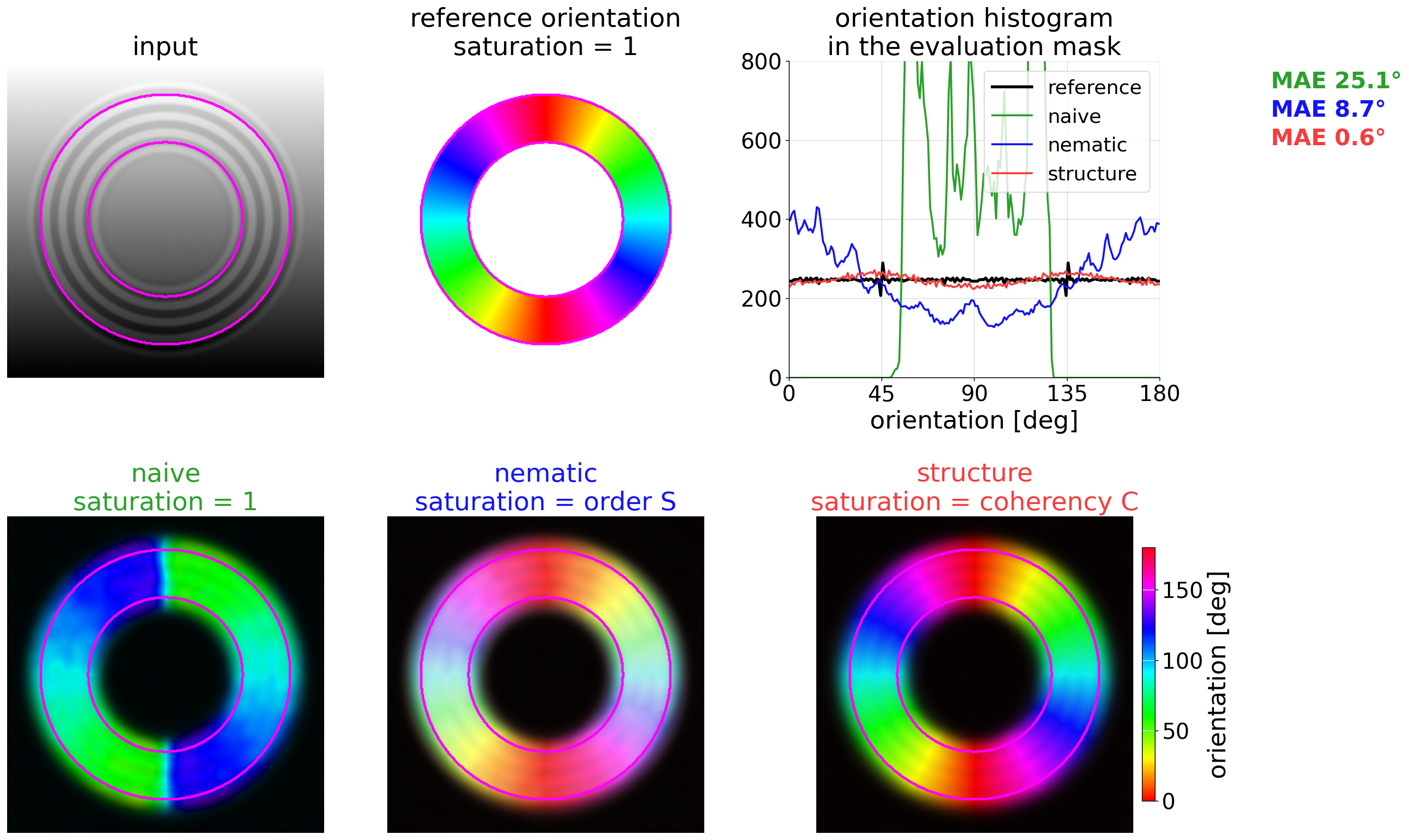
The medium level. Top: the input with the evaluation mask outlined in magenta; the reference orientation, coded as hue over the full colour circle so that 0° and 180° have the same colour; the histograms of the estimated orientation inside the mask (bins of 1°) with the MAE of each estimator. Bottom: the estimated fields as HSB maps — hue = orientation, saturation = confidence (S for the nematic tensor, C for the structure tensor, 1 for the naive mean, which has none), brightness = energy E. A colour that differs from the reference map at the same place is an orientation error. The naive mean fails around the wrap-around 0° = 180°. The nematic tensor, which gives the saturated pixels the same weight as the ring pixels, is pulled towards the ramp orientation (0°) wherever the ring orientation differs from it. The structure tensor, which weights the saturated pixels by their small gradient energy, follows the reference.

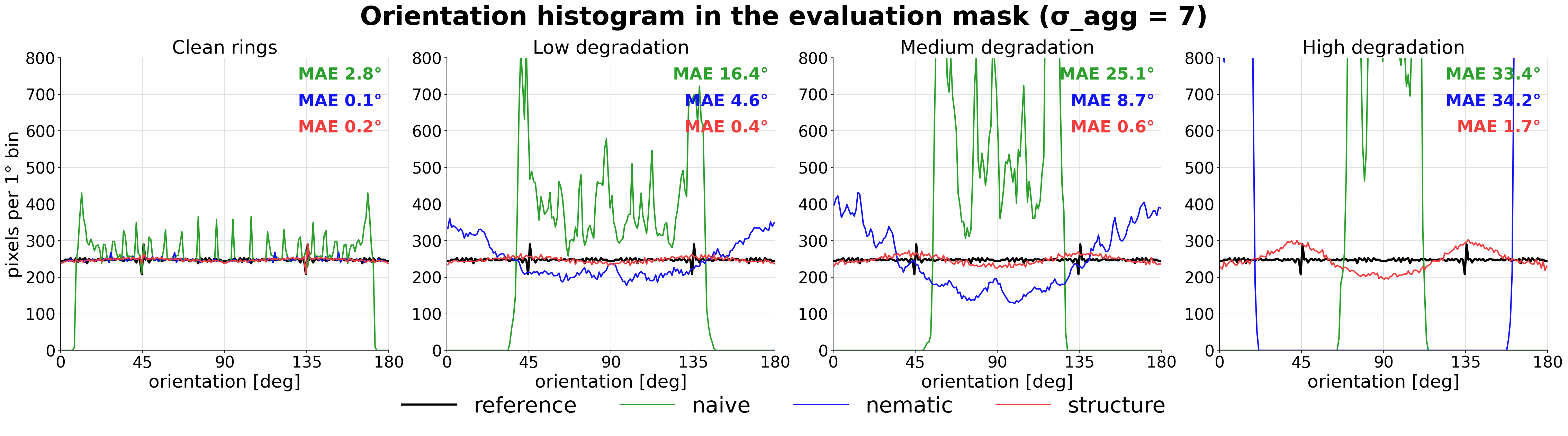
Orientation histograms in the evaluation mask at the four levels; the reference is flat. On clean rings both tensors are exact and the naive mean fails only around 0° = 180°. As the degradation grows, the nematic histogram bends towards 0° and 180°, the orientation of the ramp; the structure tensor stays flat until the high level, where the nematic tensor is no better than the naive mean.

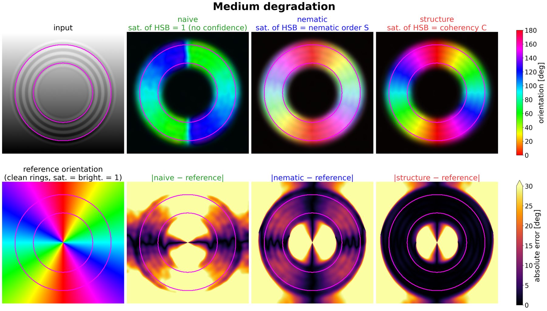
Maps at the medium level. Top: input and HSB maps. Bottom: reference orientation and absolute error of each estimator over the whole image. The nematic error is largest where the rings are far from the ramp orientation; the structure-tensor error stays within a degree.

One degradation at a time¶

The others stay at their baseline. In each figure: top, the inputs; middle, the orientation histograms of the two tensors inside the mask with their MAE; bottom, the absolute error, the confidence (S and C) and the energy E against the swept parameter (mean ± standard deviation, filled markers; median, hollow markers). The naive mean is left out.

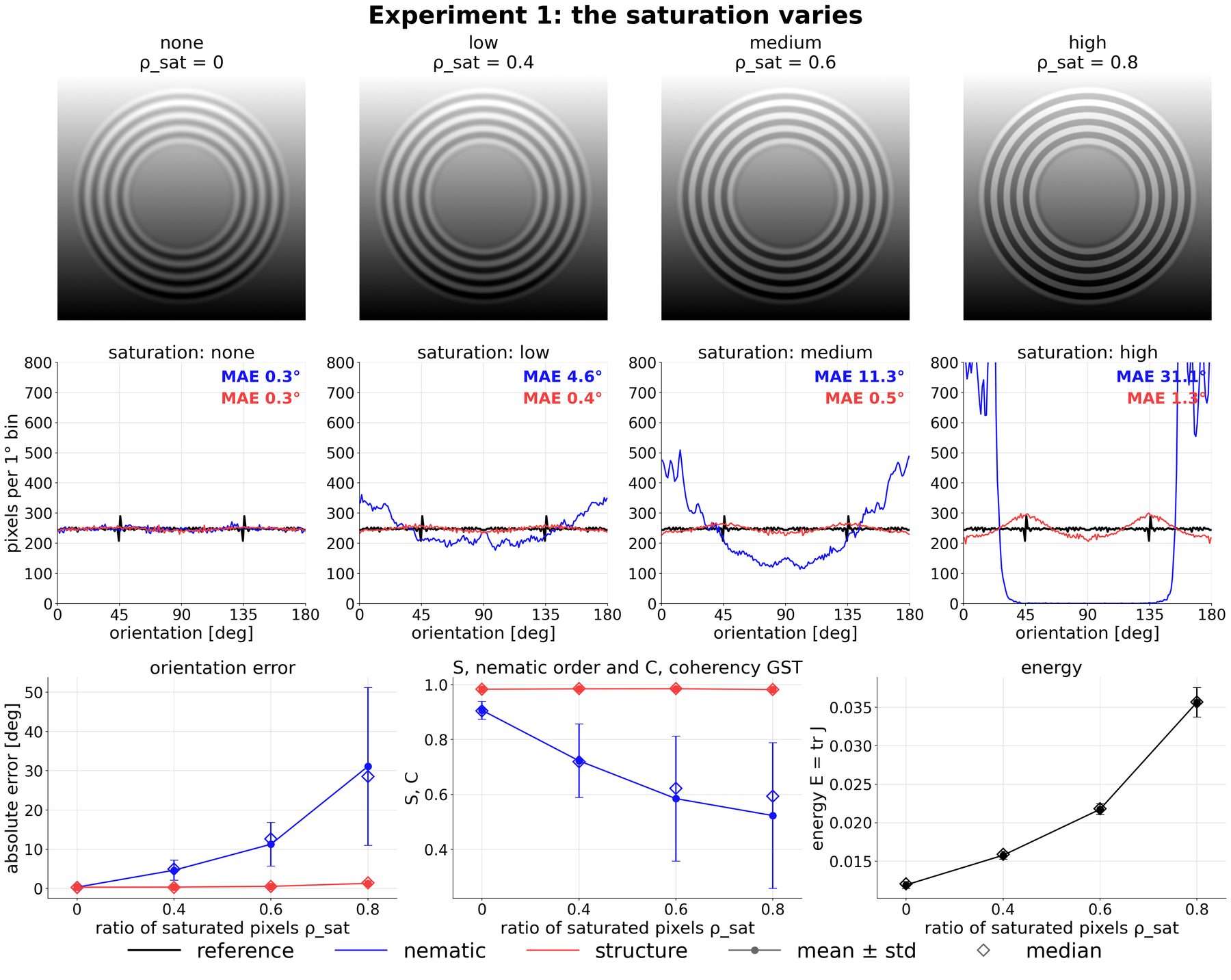
Saturation, ρ_sat = 0, 0.4, 0.6, 0.8. The nematic tensor gives every saturated pixel the weight 1, so its bias grows with the saturated fraction. The structure tensor gives them the weight of the ramp gradient, about β_ramp², and stays accurate.

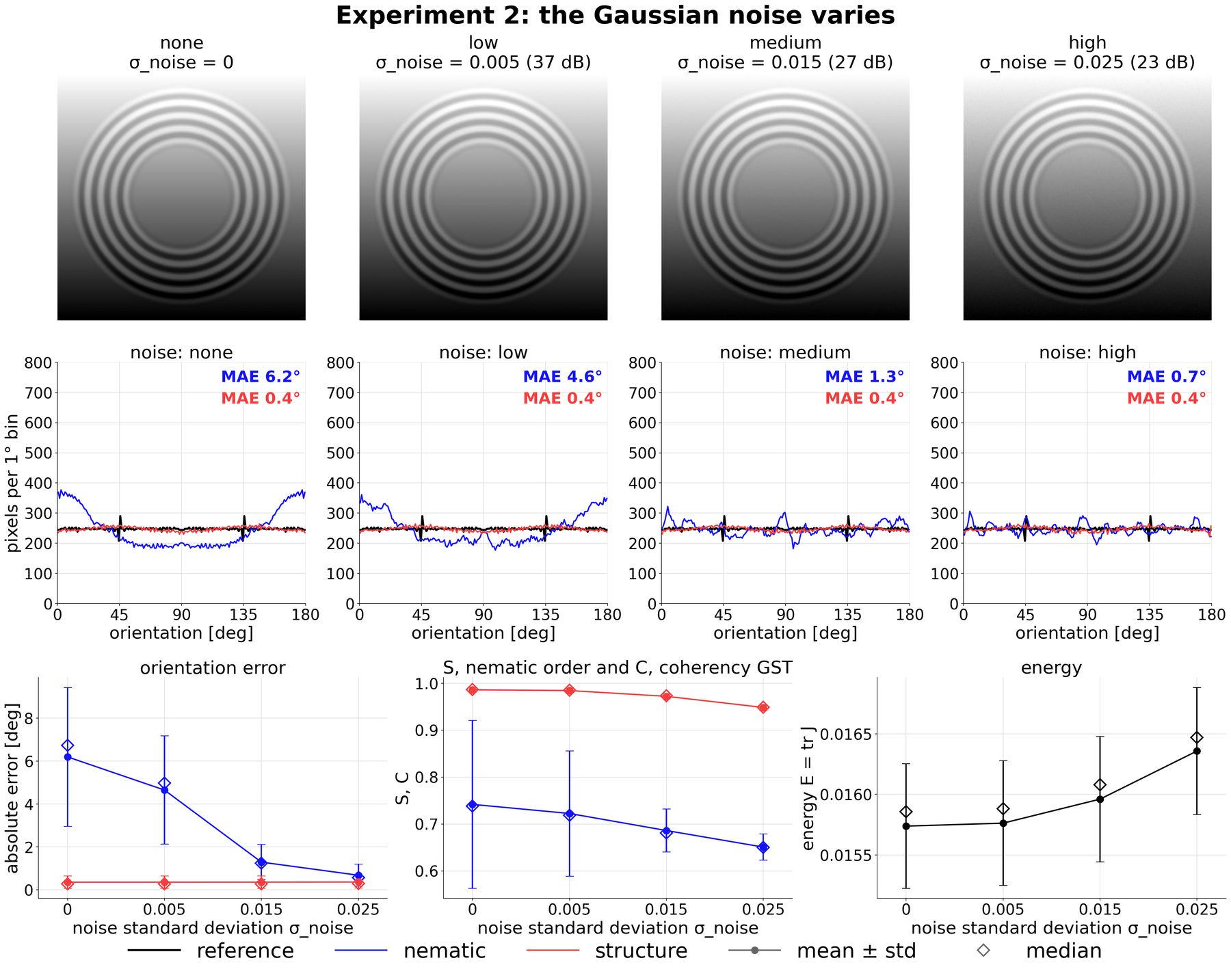
Gaussian noise, σ_noise = 0, 0.005, 0.015, 0.025. In the saturated regions the noise gradient competes with the ramp gradient. While the ramp dominates, the saturated pixels vote for the ramp orientation and bias the nematic tensor; once the noise dominates, they vote at random, the nematic bias shrinks and S drops. The structure tensor is unaffected.

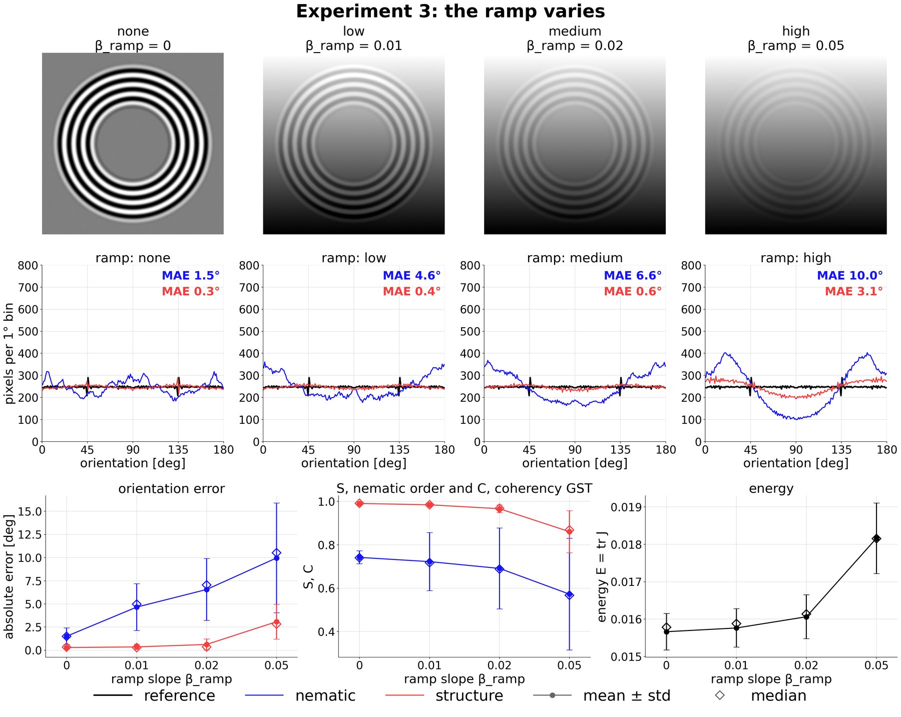
Ramp, β_ramp = 0, 0.01, 0.02, 0.05. Over a window of about one period, with ρ_sat the fraction of saturated pixels, E₁ the mean gradient energy of the rings and Δ the angle between the ramp and the reference, the biases are δ_Q = ½ atan2(ρ_sat sin 2Δ, 1 − ρ_sat + ρ_sat cos 2Δ) and δ_J = ½ atan2(κ² sin 2Δ, 1 + κ² cos 2Δ) with κ² = β_ramp²/E₁. The nematic bias appears as soon as the ramp exists and does not depend on its slope, since every saturated pixel votes for the ramp with the weight 1; the structure-tensor bias grows with β_ramp². At the high level the ramp also dominates part of the slopes and both tensors are pulled towards 0°.

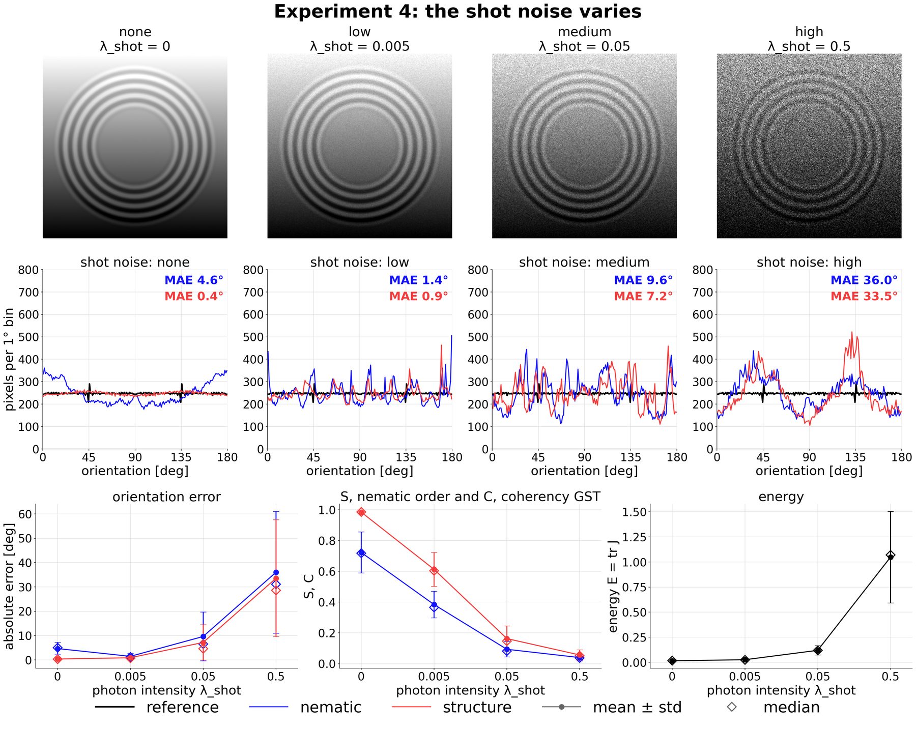
Shot noise, λ_shot = 0, 0.005, 0.05, 0.5, a noise standard deviation of about 0, 0.1, 0.3 and 1.0 in the mask, larger on the bright side of the ramp. At the low level the noise randomizes the saturated pixels and reduces the nematic bias, as with the Gaussian noise. At the medium and high levels the noise gradient exceeds the ring gradient and both tensors fail.

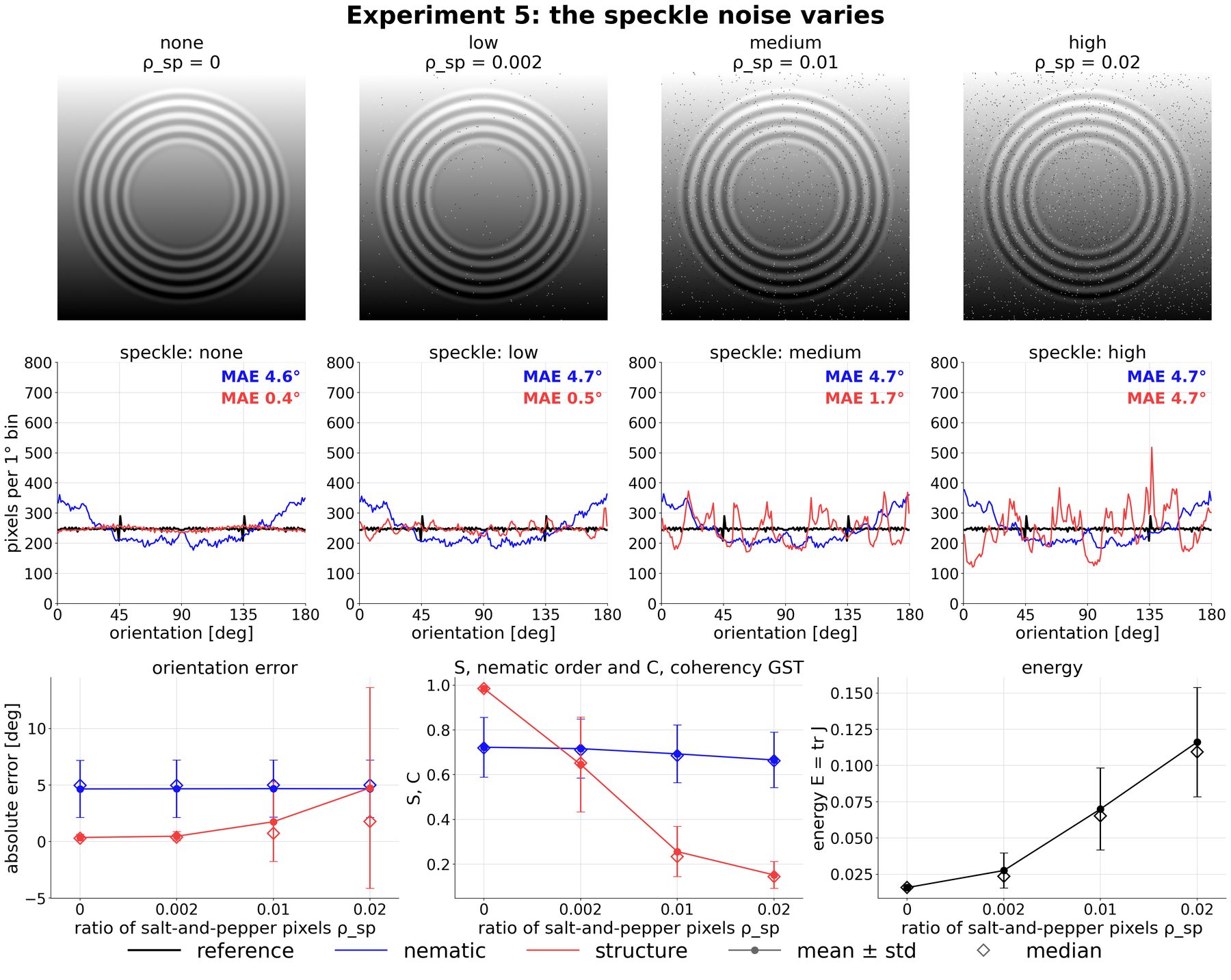
Speckle noise, ρ_sp = 0, 0.002, 0.01, 0.02. An impulse takes the maximum or the minimum of the image and changes the gradient of its four neighbours only, to about half its height, along the two axes. In the nematic tensor these four pixels weigh 1 each among some 600 in the window and their unit vectors add up to an isotropic matrix: Q does not rotate. In the structure tensor they weigh about 60 times a ring pixel; their contribution is not isotropic unless the impulse sits at the window centre, and its orientation is random. At ρ_sp = 0.01 a window holds about six impulses whose energy exceeds that of the rings: E grows, C collapses, the error rises. This is the reverse of the saturation: weighting by the energy makes the structure tensor ignore weak spurious pixels but exposes it to strong ones.

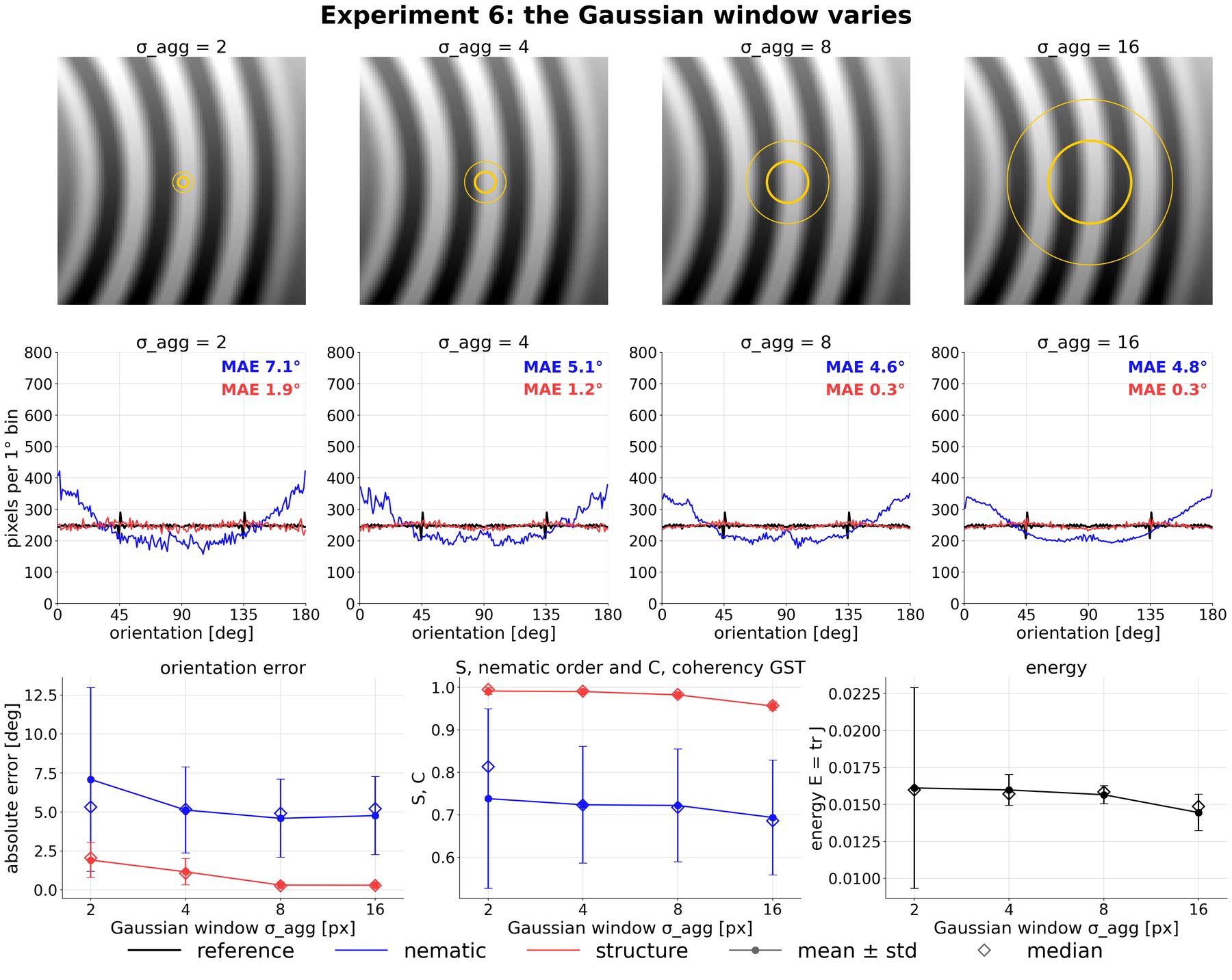
Window, σ_agg = 2, 4, 8, 16 px, against the ring period T = 20 px; the top row is a 96 × 96 px crop of the input with circles of radius σ_agg and 2σ_agg. A window smaller than one period sees single slopes or single saturated regions and makes both estimators noisier. A larger window does not remove the nematic bias.

In short¶

Since version 2.2.0 the Vector Field command of the plugin offers the three aggregations of this assessment for the pixels of a grid cell — Nematic Tensor (default), Structure Tensor, and the Simple Average of the earlier versions.

The three estimators share the gradient and the window and differ by the weight of a pixel: none, one, or its gradient energy. On clean rings the two tensors are exact and the naive mean fails at the wrap-around. Under saturation and a ramp — flat regions whose only gradient is spurious — the unit weight of the nematic tensor lets those pixels vote and biases it towards the ramp, a bias that no window size removes; the energy weight of the structure tensor silences them. The same weight exposes the structure tensor to strong impulses, which the nematic tensor ignores. Noise that randomizes the spurious pixels reduces the nematic bias but lowers its order.

Files¶

file	content
ring_experiment_lib.py	the ring image and its degradations, the three estimators, the evaluation in the mask, the drawing helpers
structure_nematic_experiment.ipynb	the experiment: the four levels, one sweep per degradation, the sweep of the window
create_abstract_figure.ipynb	the summary figure at the medium level
images/	the ring image at the four levels, 32-bit TIFF

Run with jupyter nbconvert --to notebook --execute --inplace <notebook>; needs numpy, scipy, matplotlib, tifffile.